前言

本节学习决策树

• 非参数学习算法
• 天然可以解决多分类问题
• 也可以解决回归问题

复杂度

• 训练O(nmlogm)
• 预测O(logm)

1、按熵划分的决策树

先直观感受下决策树是这个样子的
以鸢尾花数据集为例

那么决策树的划分依据是什么
主要有信息熵和基尼系数

信息熵就不多做介绍了
这里的决策是划分后使得熵降低

实现如下

import numpy as np
import matplotlib.pyplot as plt
from sklearn import datasets
from sklearn.tree import DecisionTreeClassifier
from collections import Counter
from math import log"""使用信息熵进行划分，构建决策树"""
# 数据
iris = datasets.load_iris()
X = iris.data[:, 2:]
y = iris.target
plt.scatter(X[y == 0, 0], X[y == 0, 1])
plt.scatter(X[y == 1, 0], X[y == 1, 1])
plt.scatter(X[y == 2, 0], X[y == 2, 1])
plt.show()
# 划分函数
def split(X, y, d, value):index_a = (X[:,d] <= value)index_b = (X[:,d] > value)return X[index_a], X[index_b], y[index_a], y[index_b]
# 熵
def entropy(y):counter = Counter(y)res = 0.0for num in counter.values():p = num / len(y)res += -p * log(p)return res
# 根据熵进行划分
def try_split(X, y):best_entropy = float('inf')best_d, best_v = -1, -1for d in range(X.shape[1]):sorted_index = np.argsort(X[:, d])for i in range(1, len(X)):if X[sorted_index[i], d] != X[sorted_index[i - 1], d]:v = (X[sorted_index[i], d] + X[sorted_index[i - 1], d]) / 2X_l, X_r, y_l, y_r = split(X, y, d, v)p_l, p_r = len(X_l) / len(X), len(X_r) / len(X)e = p_l * entropy(y_l) + p_r * entropy(y_r)if e < best_entropy:best_entropy, best_d, best_v = e, d, vreturn best_entropy, best_d, best_v
best_entropy, best_d, best_v = try_split(X, y)
print("best_entropy =", best_entropy)
print("best_d =", best_d)
print("best_v =", best_v)"""用scikit实现决策树"""
# 决策树，深度为2，按熵决策
dt_clf = DecisionTreeClassifier(max_depth=2, criterion="entropy", random_state=42)
dt_clf.fit(X, y)
# 决策边界可视化
def plot_decision_boundary(model, axis):x0, x1 = np.meshgrid(np.linspace(axis[0], axis[1], int((axis[1] - axis[0]) * 100)).reshape(-1, 1),np.linspace(axis[2], axis[3], int((axis[3] - axis[2]) * 100)).reshape(-1, 1),)X_new = np.c_[x0.ravel(), x1.ravel()]y_predict = model.predict(X_new)zz = y_predict.reshape(x0.shape)from matplotlib.colors import ListedColormapcustom_cmap = ListedColormap(['#EF9A9A', '#FFF59D', '#90CAF9'])plt.contourf(x0, x1, zz, cmap=custom_cmap)
plot_decision_boundary(dt_clf, axis=[0.5, 7.5, 0, 3])
plt.scatter(X[y == 0, 0], X[y == 0, 1])
plt.scatter(X[y == 1, 0], X[y == 1, 1])
plt.scatter(X[y == 2, 0], X[y == 2, 1])
plt.show()

效果如下

2、按基尼系数划分

基尼系数

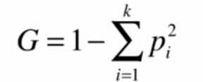
效果和按熵划分差别不大

实现如下

import numpy as np
import matplotlib.pyplot as plt
from sklearn import datasets
from sklearn.tree import DecisionTreeClassifier
from collections import Counter
from math import log"""使用基尼系数进行划分，构建决策树"""
# 数据
iris = datasets.load_iris()
X = iris.data[:, 2:]
y = iris.target
plt.scatter(X[y == 0, 0], X[y == 0, 1])
plt.scatter(X[y == 1, 0], X[y == 1, 1])
plt.scatter(X[y == 2, 0], X[y == 2, 1])
plt.show()
# 划分函数
def split(X, y, d, value):index_a = (X[:,d] <= value)index_b = (X[:,d] > value)return X[index_a], X[index_b], y[index_a], y[index_b]
# 基尼系数
def gini(y):counter = Counter(y)res = 1.0for num in counter.values():p = num / len(y)res -= p**2return res
# 根据基尼系数进行划分
def try_split(X, y):best_g = float('inf')best_d, best_v = -1, -1for d in range(X.shape[1]):sorted_index = np.argsort(X[:, d])for i in range(1, len(X)):if X[sorted_index[i], d] != X[sorted_index[i - 1], d]:v = (X[sorted_index[i], d] + X[sorted_index[i - 1], d]) / 2X_l, X_r, y_l, y_r = split(X, y, d, v)p_l, p_r = len(X_l) / len(X), len(X_r) / len(X)g = p_l * gini(y_l) + p_r * gini(y_r)if g < best_g:best_g, best_d, best_v = g, d, vreturn best_g, best_d, best_v
best_g, best_d, best_v = try_split(X, y)
print("best_g =", best_g)
print("best_d =", best_d)
print("best_v =", best_v)"""用scikit实现决策树"""
# 决策树，深度为2，按基尼系数决策
dt_clf = DecisionTreeClassifier(max_depth=2, criterion="gini", random_state=42)
dt_clf.fit(X, y)
# 决策边界可视化
def plot_decision_boundary(model, axis):x0, x1 = np.meshgrid(np.linspace(axis[0], axis[1], int((axis[1] - axis[0]) * 100)).reshape(-1, 1),np.linspace(axis[2], axis[3], int((axis[3] - axis[2]) * 100)).reshape(-1, 1),)X_new = np.c_[x0.ravel(), x1.ravel()]y_predict = model.predict(X_new)zz = y_predict.reshape(x0.shape)from matplotlib.colors import ListedColormapcustom_cmap = ListedColormap(['#EF9A9A', '#FFF59D', '#90CAF9'])plt.contourf(x0, x1, zz, cmap=custom_cmap)
plot_decision_boundary(dt_clf, axis=[0.5, 7.5, 0, 3])
plt.scatter(X[y == 0, 0], X[y == 0, 1])
plt.scatter(X[y == 1, 0], X[y == 1, 1])
plt.scatter(X[y == 2, 0], X[y == 2, 1])
plt.show()

效果如下

3、超参数

影响决策树效果的超参数

• 最大深度
• 拆分所需最小样本数
• 最大叶子数

import numpy as np
import matplotlib.pyplot as plt
from sklearn import datasets
from sklearn.tree import DecisionTreeClassifier"""超参数"""
# 数据
X, y = datasets.make_moons(noise=0.25, random_state=666)
plt.scatter(X[y == 0, 0], X[y == 0, 1])
plt.scatter(X[y == 1, 0], X[y == 1, 1])
plt.show()
# 决策树训练
dt_clf = DecisionTreeClassifier() #默认基尼系数
dt_clf.fit(X, y)
# 决策边界
def plot_decision_boundary(model, axis):x0, x1 = np.meshgrid(np.linspace(axis[0], axis[1], int((axis[1] - axis[0]) * 100)).reshape(-1, 1),np.linspace(axis[2], axis[3], int((axis[3] - axis[2]) * 100)).reshape(-1, 1),)X_new = np.c_[x0.ravel(), x1.ravel()]y_predict = model.predict(X_new)zz = y_predict.reshape(x0.shape)from matplotlib.colors import ListedColormapcustom_cmap = ListedColormap(['#EF9A9A', '#FFF59D', '#90CAF9'])plt.contourf(x0, x1, zz, linewidth=5, cmap=custom_cmap)
plot_decision_boundary(dt_clf, axis=[-1.5, 2.5, -1.0, 1.5])
plt.scatter(X[y == 0, 0], X[y == 0, 1])
plt.scatter(X[y == 1, 0], X[y == 1, 1])
plt.show()# 修改最大深度
dt_clf2 = DecisionTreeClassifier(max_depth=2)
dt_clf2.fit(X, y)
plot_decision_boundary(dt_clf2, axis=[-1.5, 2.5, -1.0, 1.5])
plt.scatter(X[y == 0, 0], X[y == 0, 1])
plt.scatter(X[y == 1, 0], X[y == 1, 1])
plt.show()# 修改最小拆分所需样本数
dt_clf3 = DecisionTreeClassifier(min_samples_split=10)
dt_clf3.fit(X, y)
plot_decision_boundary(dt_clf3, axis=[-1.5, 2.5, -1.0, 1.5])
plt.scatter(X[y == 0, 0], X[y == 0, 1])
plt.scatter(X[y == 1, 0], X[y == 1, 1])
plt.show()
dt_clf4 = DecisionTreeClassifier(min_samples_leaf=6)
dt_clf4.fit(X, y)
plot_decision_boundary(dt_clf4, axis=[-1.5, 2.5, -1.0, 1.5])
plt.scatter(X[y == 0, 0], X[y == 0, 1])
plt.scatter(X[y == 1, 0], X[y == 1, 1])
plt.show()# 修改最大叶子数
dt_clf5 = DecisionTreeClassifier(max_leaf_nodes=4)
dt_clf5.fit(X, y)
plot_decision_boundary(dt_clf5, axis=[-1.5, 2.5, -1.0, 1.5])
plt.scatter(X[y == 0, 0], X[y == 0, 1])
plt.scatter(X[y == 1, 0], X[y == 1, 1])
plt.show()

可以修改这些参数
感受过拟合和欠拟合的结果

结语

本节学习了决策树
通常都是配合其他机器学习算法使用