当前位置：首页 > news >正文

携程的网站建设/网站seo优化是什么意思

news 2025/7/28 21:16:41

携程的网站建设,网站seo优化是什么意思,creative wordpress,建网站英语1.数据集：284807 特征 31个 ，v1-v29 amoutclass( 分类 0 是非欺诈行为，1 是欺诈行为)。 2.查看样本分布规则： 0 是非欺诈行为，1 是欺诈行为。样本极度不平均解决方案： 1.下采样让0和1 样本一样小…

1.数据集：284807 特征 31个，v1-v29 +amout+class( 分类 0 是非欺诈行为，1 是欺诈行为)。
2.查看样本分布规则：
这里写图片描述
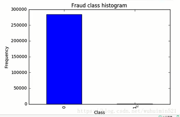
0 是非欺诈行为，1 是欺诈行为。
样本极度不平均解决方案：
1.下采样让0和1 样本一样小。同样少
2.上采样对1样本生成数据，和0 样本一样多。同样多。
amout 数值分布差异较大，采用归一或标准化。

from sklearn.preprocessing import StandardScaler
data['normAmount'] = StandardScaler().fit_transform(data['Amount'].reshape(-1, 1))
data = data.drop(['Time','Amount'],axis=1)
data.head()

采用下采样：

X = data.ix[:, data.columns != 'Class']  #取出不包括 class其他的列
print(X)
y = data.ix[:, data.columns == 'Class']  #取出包括 class这一列# Number of data points in the minority class
number_records_fraud = len(data[data.Class == 1])
fraud_indices = np.array(data[data.Class == 1].index)
print(fraud_indices)# Picking the indices of the normal classes
normal_indices = data[data.Class == 0].index# Out of the indices we picked, randomly select "x" number (number_records_fraud)
random_normal_indices = np.random.choice(normal_indices, number_records_fraud, replace = False)
random_normal_indices = np.array(random_normal_indices)# Appending the 2 indices
under_sample_indices = np.concatenate([fraud_indices,random_normal_indices])# Under sample dataset  定位
under_sample_data = data.iloc[under_sample_indices,:]X_undersample = under_sample_data.ix[:, under_sample_data.columns != 'Class']
y_undersample = under_sample_data.ix[:, under_sample_data.columns == 'Class']# Showing ratio
print("Percentage of normal transactions: ", len(under_sample_data[under_sample_data.Class == 0])/len(under_sample_data))
print("Percentage of fraud transactions: ", len(under_sample_data[under_sample_data.Class == 1])/len(under_sample_data))
print("Total number of transactions in resampled data: ", len(under_sample_data))

3.交叉验证：切分测试集和训练集

from sklearn.cross_validation import train_test_split# Whole dataset
X_train, X_test, y_train, y_test = train_test_split(X,y,test_size = 0.3, random_state = 0)print("Number transactions train dataset: ", len(X_train))
print("Number transactions test dataset: ", len(X_test))
print("Total number of transactions: ", len(X_train)+len(X_test))# Undersampled dataset
X_train_undersample, X_test_undersample, y_train_undersample, y_test_undersample = train_test_split(X_undersample,y_undersample,test_size = 0.3,random_state = 0)
print("")
print("Number transactions train dataset: ", len(X_train_undersample))
print("Number transactions test dataset: ", len(X_test_undersample))
print("Total number of transactions: ", len(X_train_undersample)+len(X_test_undersample))

对原始测试集和我们选的测试集都进行区分：
Number transactions train dataset: 199364
Number transactions test dataset: 85443
Total number of transactions: 284807

Number transactions train dataset: 688
Number transactions test dataset: 296
Total number of transactions: 984
4.模型评估
精度：数据样本分布不均，虽然很高，但很可能一个没检测出来，所以经常用recall

#Recall = TP/(TP+FN)
from sklearn.linear_model import LogisticRegression
from sklearn.cross_validation import KFold, cross_val_score
from sklearn.metrics import confusion_matrix,recall_score,classification_report

正则化惩罚：L2 正则化
机器学习中几乎都可以看到损失函数后面会添加一个额外项，常用的额外项一般有两种，一般英文称作ℓ1-norm和ℓ2-norm，中文称作L1正则化和L2正则化，或者L1范数和L2范数。

L1正则化和L2正则化可以看做是损失函数的惩罚项。所谓『惩罚』是指对损失函数中的某些参数做一些限制。对于线性回归模型，使用L1正则化的模型建叫做Lasso回归，使用L2正则化的模型叫做Ridge回归（岭回归）。下图是Python中Lasso回归的损失函数，式中加号后面一项α||w||1
即为L1正则化项。
L1正则化是指权值向量w中各个元素的绝对值之和，通常表示为||w||1
L2正则化是指权值向量w
中各个元素的平方和然后再求平方根（可以看到Ridge回归的L2正则化项有平方符号），通常表示为||w||2。一般都会在正则化项之前添加一个系数，Python中用α表示，一些文章也用λ表示。这个系数需要用户指定。

那添加L1和L2正则化有什么用？下面是L1正则化和L2正则化的作用，这些表述可以在很多文章中找到。

L1正则化可以产生稀疏权值矩阵，即产生一个稀疏模型，可以用于特征选择
L2正则化可以防止模型过拟合（overfitting）；一定程度上，L1也可以防止过拟合

def printing_Kfold_scores(x_train_data,y_train_data):fold = KFold(len(y_train_data),5,shuffle=False) # Different C parametersc_param_range = [0.01,0.1,1,10,100]results_table = pd.DataFrame(index = range(len(c_param_range),2), columns = ['C_parameter','Mean recall score'])results_table['C_parameter'] = c_param_range# the k-fold will give 2 lists: train_indices = indices[0], test_indices = indices[1]j = 0for c_param in c_param_range:print('-------------------------------------------')print('C parameter: ', c_param)print('-------------------------------------------')print('')recall_accs = []for iteration, indices in enumerate(fold,start=1):# Call the logistic regression model with a certain C parameterlr = LogisticRegression(C = c_param, penalty = 'l1')# Use the training data to fit the model. In this case, we use the portion of the fold to train the model# with indices[0]. We then predict on the portion assigned as the 'test cross validation' with indices[1]lr.fit(x_train_data.iloc[indices[0],:],y_train_data.iloc[indices[0],:].values.ravel())# Predict values using the test indices in the training datay_pred_undersample = lr.predict(x_train_data.iloc[indices[1],:].values)# Calculate the recall score and append it to a list for recall scores representing the current c_parameterrecall_acc = recall_score(y_train_data.iloc[indices[1],:].values,y_pred_undersample)recall_accs.append(recall_acc)print('Iteration ', iteration,': recall score = ', recall_acc)# The mean value of those recall scores is the metric we want to save and get hold of.results_table.ix[j,'Mean recall score'] = np.mean(recall_accs)j += 1print('')print('Mean recall score ', np.mean(recall_accs))print('')best_c = results_table.loc[results_table['Mean recall score'].idxmax()]['C_parameter']# Finally, we can check which C parameter is the best amongst the chosen.print('*********************************************************************************')print('Best model to choose from cross validation is with C parameter = ', best_c)print('*********************************************************************************')return best_c

结果如图所示：

-------------------------------------------
C parameter:  0.01
-------------------------------------------Iteration  1 : recall score =  0.958904109589
Iteration  2 : recall score =  0.917808219178
Iteration  3 : recall score =  1.0
Iteration  4 : recall score =  0.972972972973
Iteration  5 : recall score =  0.954545454545Mean recall score  0.960846151257-------------------------------------------
C parameter:  0.1
-------------------------------------------Iteration  1 : recall score =  0.835616438356
Iteration  2 : recall score =  0.86301369863
Iteration  3 : recall score =  0.915254237288
Iteration  4 : recall score =  0.932432432432
Iteration  5 : recall score =  0.878787878788Mean recall score  0.885020937099-------------------------------------------
C parameter:  1
-------------------------------------------Iteration  1 : recall score =  0.835616438356
Iteration  2 : recall score =  0.86301369863
Iteration  3 : recall score =  0.966101694915
Iteration  4 : recall score =  0.945945945946
Iteration  5 : recall score =  0.893939393939Mean recall score  0.900923434357-------------------------------------------
C parameter:  10
-------------------------------------------Iteration  1 : recall score =  0.849315068493
Iteration  2 : recall score =  0.86301369863
Iteration  3 : recall score =  0.966101694915
Iteration  4 : recall score =  0.959459459459
Iteration  5 : recall score =  0.893939393939Mean recall score  0.906365863087-------------------------------------------
C parameter:  100
-------------------------------------------Iteration  1 : recall score =  0.86301369863
Iteration  2 : recall score =  0.86301369863
Iteration  3 : recall score =  0.966101694915
Iteration  4 : recall score =  0.959459459459
Iteration  5 : recall score =  0.893939393939Mean recall score  0.909105589115*********************************************************************************
Best model to choose from cross validation is with C parameter =  0.01
*********************************************************************************

6.混淆矩阵
下采样问题：误差太多了。
https://blog.csdn.net/fjssharpsword/article/details/79104071

def plot_confusion_matrix(cm, classes,title='Confusion matrix',cmap=plt.cm.Blues):"""This function prints and plots the confusion matrix."""plt.imshow(cm, interpolation='nearest', cmap=cmap)plt.title(title)plt.colorbar()tick_marks = np.arange(len(classes))plt.xticks(tick_marks, classes, rotation=0)plt.yticks(tick_marks, classes)thresh = cm.max() / 2.for i, j in itertools.product(range(cm.shape[0]), range(cm.shape[1])):plt.text(j, i, cm[i, j],horizontalalignment="center",color="white" if cm[i, j] > thresh else "black")plt.tight_layout()plt.ylabel('True label')plt.xlabel('Predicted label')plt.show()
import itertools
lr = LogisticRegression(C = best_c, penalty = 'l1')
lr.fit(X_train_undersample,y_train_undersample.values.ravel())
y_pred_undersample = lr.predict(X_test_undersample.values)# Compute confusion matrix
cnf_matrix = confusion_matrix(y_test_undersample,y_pred_undersample)
np.set_printoptions(precision=2)print("Recall metric in the testing dataset: ", cnf_matrix[1,1]/(cnf_matrix[1,0]+cnf_matrix[1,1]))# Plot non-normalized confusion matrix
class_names = [0,1]
plt.figure()
plot_confusion_matrix(cnf_matrix, classes=class_names, title='Confusion matrix')
plt.show()

7.threshold 参数
调整逻辑回归阈值看哪个参数最合适，可以调整。

lr = LogisticRegression(C = 0.01, penalty = 'l1')
lr.fit(X_train_undersample,y_train_undersample.values.ravel())
y_pred_undersample_proba = lr.predict_proba(X_test_undersample.values)thresholds = [0.1,0.2,0.3,0.4,0.5,0.6,0.7,0.8,0.9]plt.figure(figsize=(10,10))j = 1
for i in thresholds:y_test_predictions_high_recall = y_pred_undersample_proba[:,1] > iplt.subplot(3,3,j)j += 1# Compute confusion matrixcnf_matrix = confusion_matrix(y_test_undersample,y_test_predictions_high_recall)np.set_printoptions(precision=2)print("Recall metric in the testing dataset: ", cnf_matrix[1,1]/(cnf_matrix[1,0]+cnf_matrix[1,1]))# Plot non-normalized confusion matrixclass_names = [0,1]plot_confusion_matrix(cnf_matrix, classes=class_names, title='Threshold >= %s'%i)