wordpress 整站打包/网站推广的作用

点击蓝字关注我哦
 人脸识别的过程,其实就是一个人脸照片和姓名匹配的过程,也就是将一些混乱的图片给分类,贴上对应的姓名。模型越好,分类的效果最好,越熟悉的人,越容易在人群中一眼认出来,大概最高的熟悉程度是化成灰都认识吧。
一、使用LFW数据库作为训练的数据集

from sklearn.datasets import fetch_lfw_peoplefaces = fetch_lfw_people(min_faces_per_person=60)print(faces.target_names)print(faces.images.shape)fetch_lfw_people: load the labeled faces in the Wild(LFW) people dataset(classification).
这篇短文中使用的人脸数据样本来自于”Labeled Faces in the Wild (LFW)”,这是一个用于学习人脸识别问题的人脸照片数据库。这个数据库由University of Massachusetts的研究员Amherst创立和维护,数据库中包含5749个人的13233张图片。
换句话说dataset里面含有的classes有5749个,一共有13233个samples, dimensionality:5828个,features:0-255(用来表示颜色的参数R G B三原色每个参数取值范围都是0-255)
min_faces_per_person:提取的数据集中每个人将保留具有至少有min_faces_per_person个不同图片。Returns: 返回的faces包含下面的四项内容:
data(13233,2914):返回的data那个矩阵shape为13233x2914,每一行对应一个原始尺寸为62x47的人脸图像images(13233,62,47):每一行对应5749个人中某一个人的人脸图像数据。
target(13233,):每一个人脸图像对应的标签,从0到5478,一个数字对应一个人的ID。
Target_Names:target中的每个人的ID对应的个人的姓名,将个人ID和个人姓名一一对应起来。
DESCR:一段关于LFW数据库的描述性文字。
import matplotlib.pyplot as pltfig, ax = plt.subplots(3, 5) #产生三行五列个subplot.for i, axi in enumerate(ax.flat): axi.imshow(faces.images[i], cmap='bone') axi.set(xticks=[], yticks=[], xlabel=faces.target_names[faces.target[i]])plt.show()
举个小例子:
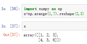
我们产生一个2行3列的array:
然后我们用list() function分别列出这个array以及这个array.flat之后的结果:
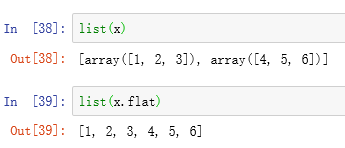
很明显的差别,x.flat之后它变成了一个一维的iterator, iterator is an object which used to iterate over an iterable object.
Enumerate() 是python的一个build-in(内建) function,它给传入的值自动从零开始编号,例如:
for i, j in enumerate(['I','love','you','my','babe']): print(i,j)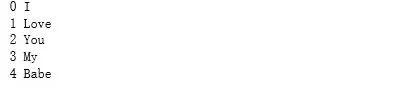
matplotlib.axes.Axes.imshow(self, X, cmap=None, norm=None, aspect=None, interpolation=None, alpha=None, vmin=None, vmax=None, origin=None, extent=None, *, filternorm=True, filterrad=4.0, resample=None, url=None, data=None, **kwargs)
 X:array-like,矩阵形式,支持的shape有:(M,N):具有标量数据的图像,使用规范化和颜色图将值映射到颜色。有不同的映射方法,norm,cmap,vmin,vmax等。对于RGB数据,将忽略此参数。(M,N,3):关于图片的数据使用的是RGB值(0-1的float(单精度浮点型)格式或者是0-255的int(整型)格式)。(M,N,4):关于图片的数据使用的是RGBA值(0-1的float格式或者是0-255的int格式),这个还包括透明度。
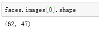
可以看到从LFW数据库提取的部分faces中第一个图片的形状是(62,47)为(M,N)的形式。
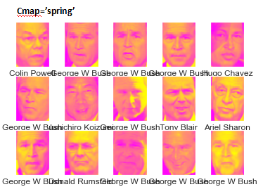
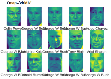
Cmap:The colormap instance or registered colormap name used to map scalar data to colors.用来将标量数据映射到颜色的颜色图实例或者已经注册过的颜色图名字, Default='viridis'。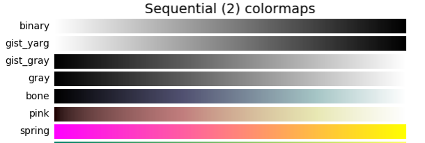

https://matplotlib.org/3.1.0/tutorials/colors/colormaps.html#mycarta-banding
Norm:在使用cmap映射之前将数据normalize为[0,1]。Vmin,vmax:当使用的数据没有明确的准则时,不知道是[0,255]还是[0,1],vmin和vmax就可以用来定义颜色图覆盖的数据范围。使用Axes.imshow(X,cmap=None)在对应的i的位置展示图片。使用set设置一些x轴刻度,y轴刻度,当然这里是空的,但是x轴的xlabel对应的是每个faces的名字,前面说到的faces.target_names里面存储了每个ID对应的名字,而target里面存的是每个图片对应的ID,这样一步步代进去,那么在每个subplot的图片下面就显示出了该图片对应的名字。
二、使用PCA提取主成分,再使用SVC进行模型训练及分类
from sklearn.svm import SVCfrom sklearn.decomposition import PCAmodel = make_pipeline(pca, svc)from sklearn.pipeline import make_pipelinepca = PCA(n_components=150, whiten=True, random_state=42)svc = SVC(kernel='rbf', class_weight='balanced')sklearn.pipeline.make_pipeline(*steps, **kwargs)
Construct a pipeline from the given estimators. 建立一个管道,里面含有一个个算子,就像是生产产品的流水线,从原始材料,经过一道道工序,变成我们想要的产品。
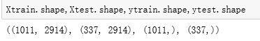
Make_pipeline(pca,svc)意思就是先使用PCA对于我们输入进去的数据进行主成分分析(Principal Component Analysis),提取比较有影响力,更能决定结果的特征,对那些无关紧要的特征和噪音过滤掉,然后再使用SVC(支持向量机)进行分类训练。from sklearn.model_selection import train_test_splitXtrain, Xtest, ytrain, ytest = train_test_split(faces.data, faces.target,random_state=42)sklearn.model_selection.train_test_split(*arrays, **options)
train_test_split是随机将所有的数据集分成训练集和测试集这两组子集,与前面"一维卷积神经网络应用于电信号分类Ⅰ"所讲的 StratifiedShuffleSplit 用法有些区别;后者先将数据集随机分成若干组,每一个组里面都包含train和test两部分,这两部分也是随机分的,但是这个train和test的比例是可以通过参数确定的,具体可以翻到那篇文章看看哈;而前者只是随机分成了train和test两部分,我们打印出来他们的shape可以看见,train里面有1011行,test里面有337行。
三、使用GridSearchCV选取最优参数
from sklearn.model_selection import GridSearchCVparam_grid = {'svc__C': [1, 5, 10, 50], 'svc__gamma': [0.0001, 0.0005, 0.001, 0.005]}grid = GridSearchCV(model, param_grid)%time grid.fit(Xtrain, ytrain)print(grid.best_params_)sklearn.model_selection.GridSearchCV(estimator, param_grid, *, scoring=None, n_jobs=None, iid='deprecated', refit=True, cv=None, verbose=0, pre_dispatch='2*n_jobs', error_score=nan, return_train_score=False)
sklearn.model_selection.GridSearchCV()详尽地搜索了estimator的指定参数,其中指定的参数存放在param_grid中。
Estimator: 所使用的 estimator, 使用的 estimator 里面需要有 scoring function,因为会通过这个scoring 最后来评价你给定的参数中哪个是最好的。
Param_grid:dict的形式,key为你的参数名字,然后参数放在list里面。下面这个样子,给SVC的C值取值范围为[1,5,10,50],SVC的gamma取值范围为[0.0001,0.0005,0.001,005],SVC的C和gamma值是啥意思,上一篇有讲到哈,参考支持向量机SVM(Support Vector Machine) Ⅰ。
param_grid = {'svc__C': [1, 5, 10, 50], 'svc__gamma': [0.0001, 0.0005, 0.001, 0.005]}
%time jupyter built-in magic commands之一,之前我们用过的%matplotlib inline也是一个magic commands, %time是用来计算你的CPU执行后面这窜代码(grid.fit(Xtrain, ytrain)所用的时间(25.3s)。
print出来最优的的参数如下: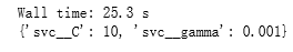
最后取C值为10,gamma值为0.001时,模型的得分是最高的。
下面使用最优的模型进行predict:
model = grid.best_estimator_yfit = model.predict(Xtest)四、检验模型的预测结果与实际结果
fig, ax = plt.subplots(4, 6)for i, axi in enumerate(ax.flat): axi.imshow(Xtest[i].reshape(62, 47), cmap='bone') axi.set(xticks=[], yticks=[]) axi.set_ylabel(faces.target_names[yfit[i]].split()[-1], color='black' if yfit[i] == ytest[i] else 'red')fig.suptitle('Predicted Names; Incorrect Labels in Red', size=14)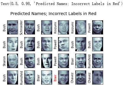 预测的name和原来的name是一样的那么用黑色字体,else用红色字体,上面看出有一个预测错误的结果。建立一个显示主要分类指标的文本报告。
from sklearn.metrics import classification_reportprint(classification_report(ytest, yfit,target_names=faces.target_names))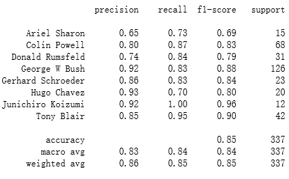
sklearn.metrics.classification_report(y_true, y_pred, *, labels=None, target_names=None, sample_weight=None, digits=2, output_dict=False, zero_division='warn')
Y_true: 就是前面把数据split的时候得到的ytest那一列数据。
Y_pred:使用你最优化模型之后预测得到的yfit值。Target_names:展示对应的标签的名字,如果没有加这个参数,那么左边这一列名字就会是一串数字,如下图。from sklearn.metrics import classification_reportprint(classification_report(ytest,yfit)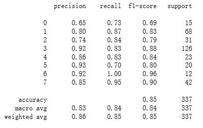
from sklearn.metrics import confusion_matriximport seaborn as sns; sns.set()mat = confusion_matrix(ytest, yfit)sns.heatmap(mat.T, square=True, annot=True, fmt='d', cbar=False, xticklabels=faces.target_names, yticklabels=faces.target_names)plt.xlabel('true label')plt.ylabel('predicted label')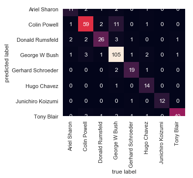
sklearn.metrics.confusion_matrix(y_true, y_pred, *, labels=None, sample_weight=None, normalize=None)
通过计算Confusion_matrix来评估分类的准确性。
Y_true: 就是前面把数据split的时候得到的ytest那一列数据。
Y_pred:使用你最优化模型之后预测得到的yfit值。
seaborn.heatmap(data, vmin=None, vmax=None, cmap=None, center=None, robust=False, annot=None, fmt='.2g', annot_kws=None, linewidths=0, linecolor='white', cbar=True, cbar_kws=None, cbar_ax=None, square=False, xticklabels='auto', yticklabels='auto', mask=None, ax=None, **kwargs)
画一个有颜色的矩阵数据,Data:矩形数据集,2D dataset.Square:为True时,x,y轴方向上大小相等,使得热力图里面的小方块每块都是正方形。这都是一些作图的参数,很好理解的,可以参考下面的文档:https://seaborn.pydata.org/generated/seaborn.heatmap.html上面的图片展示不完整,可以自己设置一下y轴的取值就显示完整了,代码如下:from sklearn.metrics import confusion_matriximport seaborn as sns; sns.set()mat = confusion_matrix(ytest, yfit)ax=sns.heatmap(mat.T, square=True, annot=True, fmt='d', cbar=False,xticklabels=faces.target_names,yticklabels=faces.target_names)plt.xlabel('true label')plt.ylabel('predicted label')ax.set_ylim([0,8])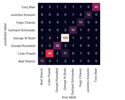


往期推荐
支持向量机SVM(Support Vector Machine) Ⅰ
一维卷积神经网络应用于电信号分类 Ⅰ
时间序列分析方法预测未来Ⅰ

点亮在看,你最好看