网站循环滚动图片z怎么做/百度游戏客服在线咨询

原文：

https://www.jianshu.com/p/00ef5b63dfc8Python数据处理从零开始----第四章（可视化）(11)多分类ROC曲线https://www.jianshu.com/p/00ef5b63dfc8

===============================================
用于评估分类器分类质量的ROC示例。

ROC曲线通常在Y轴上具有真阳性率，在X轴上具有假阳性率。这意味着图的左上角是“理想”点 - 误报率为零，真正的正率为1。这不太现实，但它确实意味着曲线下面积（AUC）通常更好。

多分类设置

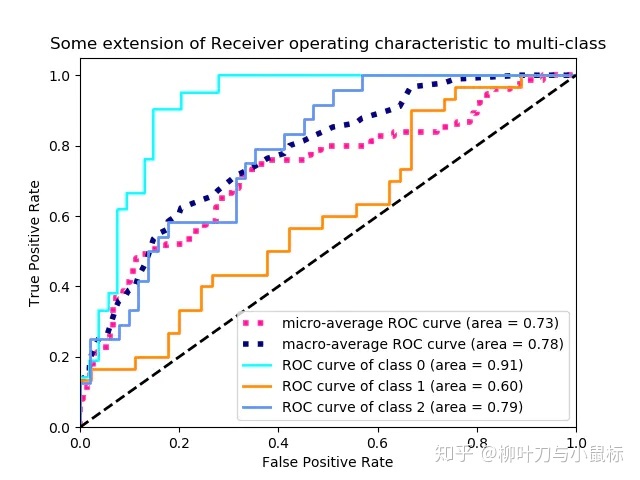
ROC曲线通常用于二分类以研究分类器的输出。为了将ROC曲线和ROC区域扩展到多类或多标签分类，有必要对输出进行二值化。⑴可以每个标签绘制一条ROC曲线。⑵也可以通过将标签指示符矩阵的每个元素视为二元预测（微平均）来绘制ROC曲线。⑶另一种用于多类别分类的评估方法是宏观平均，它对每个标签的分类给予相同的权重。

• 第一步导入所需要的包

# -*- coding: utf-8 -*- """ Created on Sun Nov 25 14:24:20 2018 @author: czh """ %clear %reset -f # In[*] import pyupset as pyu from pickle import load import os os.chdir('D:train') import numpy as np import matplotlib.pyplot as plt from itertools import cycle from sklearn import svm, datasets from sklearn.metrics import roc_curve, auc from sklearn.model_selection import train_test_split from sklearn.preprocessing import label_binarize from sklearn.multiclass import OneVsRestClassifier from scipy import interp

• 第二步导入所需要数据，本文所使用的是最常见的iris数据，预测输出变量是种类species，包含三种种类。

# In[*] # Import some data to play with iris = datasets.load_iris() X = iris.data y = iris.target # Binarize the output y = label_binarize(y, classes=[0, 1, 2]) n_classes = y.shape[1]

• 第三步建立预测模型，这里使用的是支持向量机模型。

# Add noisy features to make the problem harder random_state = np.random.RandomState(0) n_samples, n_features = X.shape X = np.c_[X, random_state.randn(n_samples, 200 * n_features)] # shuffle and split training and test sets X_train, X_test, y_train, y_test = train_test_split(X, y, test_size=.5, random_state=0) # Learn to predict each class against the other classifier = OneVsRestClassifier(svm.SVC(kernel='linear', probability=True, random_state=random_state)) y_score = classifier.fit(X_train, y_train).decision_function(X_test)

• 第四步将每一个预测点的分类都视作一个结果。

比如100个样本三分类，就出现300个二分类结果。

# Compute ROC curve and ROC area for each class fpr = dict() tpr = dict() roc_auc = dict() for i in range(n_classes): fpr[i], tpr[i], _ = roc_curve(y_test[:, i], y_score[:, i]) roc_auc[i] = auc(fpr[i], tpr[i]) # Compute micro-average ROC curve and ROC area fpr["micro"], tpr["micro"], _ = roc_curve(y_test.ravel(), y_score.ravel()) roc_auc["micro"] = auc(fpr["micro"], tpr["micro"])

• 第五步绘图

# In[*] plt.figure() lw = 2 plt.plot(fpr[2], tpr[2], color='darkorange', lw=lw, label='ROC curve (area = %0.2f)' % roc_auc[2]) plt.plot([0, 1], [0, 1], color='navy', lw=lw, linestyle='--') plt.xlim([0.0, 1.0]) plt.ylim([0.0, 1.05]) plt.xlabel('False Positive Rate') plt.ylabel('True Positive Rate') plt.title('Receiver operating characteristic example') plt.legend(loc="lower right") plt.show()

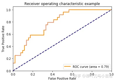
• 结论：这样我们就得到多分类情况下微观的平均ROC值

# Compute macro-average ROC curve and ROC area # First aggregate all false positive rates all_fpr = np.unique(np.concatenate([fpr[i] for i in range(n_classes)])) # Then interpolate all ROC curves at this points mean_tpr = np.zeros_like(all_fpr) for i in range(n_classes): mean_tpr += interp(all_fpr, fpr[i], tpr[i]) # Finally average it and compute AUC mean_tpr /= n_classes fpr["macro"] = all_fpr tpr["macro"] = mean_tpr roc_auc["macro"] = auc(fpr["macro"], tpr["macro"]) # Plot all ROC curves plt.figure() plt.plot(fpr["micro"], tpr["micro"], label='micro-average ROC curve (area = {0:0.2f})' ''.format(roc_auc["micro"]), color='deeppink', linestyle=':', linewidth=4) plt.plot(fpr["macro"], tpr["macro"], label='macro-average ROC curve (area = {0:0.2f})' ''.format(roc_auc["macro"]), color='navy', linestyle=':', linewidth=4) colors = cycle(['aqua', 'darkorange', 'cornflowerblue']) for i, color in zip(range(n_classes), colors): plt.plot(fpr[i], tpr[i], color=color, lw=lw, label='ROC curve of class {0} (area = {1:0.2f})' ''.format(i, roc_auc[i])) plt.plot([0, 1], [0, 1], 'k--', lw=lw) plt.xlim([0.0, 1.0]) plt.ylim([0.0, 1.05]) plt.xlabel('False Positive Rate') plt.ylabel('True Positive Rate') plt.title('Some extension of Receiver operating characteristic to multi-class') plt.legend(loc="lower right") plt.show()