当前位置：首页 > news >正文

网站空间到期时间查询/微信朋友圈营销方案

news 2025/8/13 17:38:17

网站空间到期时间查询,微信朋友圈营销方案,网站建设会议讲话,企业电子网站的建设案例写在前面： 我是「nicedays」，一枚喜爱做特效，听音乐，分享技术的大数据开发猿。这名字是来自world order乐队的一首HAVE A NICE DAY。如今，走到现在很多坎坷和不顺，如今终于明白nice day是需要自己赋予的。白…

写在前面： 我是「nicedays」，一枚喜爱做特效，听音乐，分享技术的大数据开发猿。这名字是来自world order乐队的一首HAVE A NICE DAY。如今，走到现在很多坎坷和不顺，如今终于明白nice day是需要自己赋予的。白驹过隙，时光荏苒，珍惜当下~~
写博客一方面是对自己学习的一点点总结及记录，另一方面则是希望能够帮助更多对大数据感兴趣的朋友。如果你也对 大数据与机器学习感兴趣，可以关注我的动态 https://blog.csdn.net/qq_35050438，让我们一起挖掘数据与人工智能的价值~

文章目录

- 用户画像
  - 概念：
  - 如何建立画像--根据数据：
    - 用户数据分类：
      - 静态数据：
      - 动态数据：
  - 用户画像应用：
  - 用户画像整体流程：
    - 1.数据预处理
    - 2.特征选择
    - 3. 建立模型
  - 用户画像实战案例：对用户搜词信息进行标签化
    - 一：将原始数据转换成utf-8编码，防止后续出现各种编码问题
    - 二：生成对应的数据表
    - 三：对用户的搜索数据进行分词与词性过滤
    - 四：使用Gensim库建立word2vec词向量模型
      - 参数定义：
    - 五：加载训练好的word2vec模型，求用户搜索结果的平均向量
    - 六：绘图函数，以性别为例，绘制混淆矩阵
    - 七：测试集的构造方法和训练集一样
    - 八：检查一下数据有木有问题
    - 九：建立一个基础预测模型
    - 十：堆叠模型

用户画像

概念：

Persona是真实用户的虚拟代表是建立在一系列真实数据之上的目标用户模型。
根据用户的目标，行为和观点的差异，将他们区分为不同的类型每种类型中抽取典型特征，形成了一个任务原型。
—用户信息标签化

如何建立画像—根据数据：

用户数据分类：

静态数据：

用户相对稳定的信息，如性别，地域

动态数据：

用户不停变化的行为信息，如何浏览网页，搜索商品

用户画像应用：

推荐系统，猜你喜欢
精准营销，锁定用户，广告投放

用户画像整体流程：

基于用户搜索关键词数据为用户打上标签(学历，年龄，性别)

1.数据预处理

编码方式转换
对数据搜索内容进行分词
词性过滤
数据检查

2.特征选择

建立word2vec词向量模型
对所有搜索数据求平均向量

3. 建立模型

不同机器学习模型对比
堆叠模型

用户画像实战案例：对用户搜词信息进行标签化

一：将原始数据转换成utf-8编码，防止后续出现各种编码问题

import csv#原始数据存储路径data_path = './data/user_tag_query.10W.TRAIN' #生成数据路径csvfile = open(data_path + '-1w.csv', 'w')
writer = csv.writer(csvfile)
writer.writerow(['ID', 'age', 'Gender', 'Education', 'QueryList'])#转换成utf-8编码的格式with open(data_path, 'r',encoding='gb18030',errors='ignore') as f:lines = f.readlines()    for line in lines[0:10000]:        try:line.strip()          data = line.split("\t")writedata = [data[0], data[1], data[2], data[3]]querystr = ''data[-1]=data[-1][:-1]            for d in data[4:]:                try:cur_str = d.encode('utf8')cur_str = cur_str.decode('utf8')querystr += cur_str + '\t'except:                    continue#print (data[0][0:10])querystr = querystr[:-1]writedata.append(querystr)writer.writerow(writedata)        except:            #print (data[0][0:20])continue

测试集的编码转换方式同上

data_path = './data/user_tag_query.10W.TEST'csvfile = open(data_path + '-1w.csv', 'w')
writer = csv.writer(csvfile)
writer.writerow(['ID', 'QueryList'])with open(data_path, 'r',encoding='gb18030',errors='ignore') as f:lines = f.readlines()    for line in lines[0:10000]:        try:data = line.split("\t")writedata = [data[0]]querystr = ''data[-1]=data[-1][:-1]            for d in data[1:]:                try:                  cur_str = d.encode('utf8')cur_str = cur_str.decode('utf8')querystr += cur_str + '\t'               except:                    #print (data[0][0:10])continuequerystr = querystr[:-1]writedata.append(querystr)writer.writerow(writedata)        except:            #print (data[0][0:20])continue

二：生成对应的数据表

import pandas as pd#编码转换完成的数据，取的是1W的子集trainname = './data/user_tag_query.10W.TRAIN-1w.csv'testname = './data/user_tag_query.10W.TEST-1w.csv'data = pd.read_csv(trainname,encoding='gbk')print (data.info())#分别生成三种标签数据(性别，年龄，学历)data.age.to_csv("./data/train_age.csv", index=False)
data.Gender.to_csv("./data/train_gender.csv", index=False)
data.Education.to_csv("./data/train_education.csv", index=False)#将搜索数据单独拿出来data.QueryList.to_csv("./data/train_querylist.csv", index=False)data = pd.read_csv(testname,encoding='gbk')print (data.info())data.QueryList.to_csv("./data/test_querylist.csv", index=False)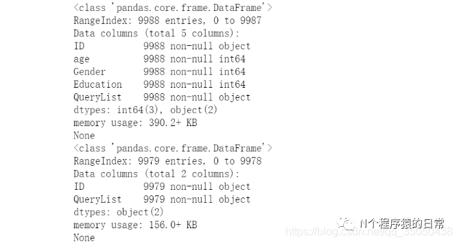

三：对用户的搜索数据进行分词与词性过滤

这里需要分别对训练集和测试集进行相同的操作，路径名字要改动一下

import pandas as pdimport jieba.analyseimport timeimport jiebaimport jieba.possegimport os, sysdef input(trainname):traindata = []    with open(trainname, 'rb') as f:line = f.readline()count = 0while line:            try:traindata.append(line)count += 1except:                print ("error:", line, count)line=f.readline()    return traindata
start = time.clock()filepath = './data/test_querylist.csv'QueryList = input(filepath)writepath = './data/test_querylist_writefile-1w.csv'csvfile = open(writepath, 'w')POS = {}for i in range(len(QueryList)):    #print (i)if i%2000 == 0 and i >=1000:        print (i,'finished') s = []str = ""words = jieba.posseg.cut(QueryList[i])# 带有词性的精确分词模式allowPOS = ['n','v','j']    for word, flag in words:POS[flag]=POS.get(flag,0)+1if (flag[0] in allowPOS) and len(word)>=2:str += word + " "cur_str = str.encode('utf8')cur_str = cur_str.decode('utf8')s.append(cur_str)csvfile.write(" ".join(s)+'\n')
csvfile.close()end = time.clock()print ("total time: %f s" % (end - start))

四：使用Gensim库建立word2vec词向量模型

参数定义：

sentences：可以是一个list
sg：用于设置训练算法，默认为0，对应CBOW算法；sg=1则采用skip-gram算法。
size：是指特征向量的维度，默认为100。大的size需要更多的训练数据,但是效果会更好. 推荐值为几十到几百。
window：表示当前词与预测词在一个句子中的最大距离是多少
alpha:是学习速率
seed：用于随机数发生器。与初始化词向量有关。
min_count:可以对字典做截断. 词频少于min_count次数的单词会被丢弃掉, 默认值为5
max_vocab_size:设置词向量构建期间的RAM限制。如果所有独立单词个数超过这个，则就消除掉其中最不频繁的一个。每一千万个单词需要大约1GB的RAM。设置成None则没有限制。
workers参数控制训练的并行数。
hs:如果为1则会采用hierarchica·softmax技巧。如果设置为0(defau·t)，则negative sampling会被使用。
negative:如果>0,则会采用negativesamp·ing，用于设置多少个noise words
iter： 迭代次数，默认为5

from gensim.models import word2vec#将数据变换成list of list格式train_path = './data/train_querylist_writefile-1w.csv'with open(train_path, 'r') as f:My_list = []lines = f.readlines()    for line in lines:cur_list = []line = line.strip()data = line.split(" ")        for d in data:cur_list.append(d)My_list.append(cur_list)model = word2vec.Word2Vec(My_list, size=300, window=10,workers=4)  savepath = '1w_word2vec_' + '300'+'.model' # 保存model的路径model.save(savepath)

测试

model.most_similar("大哥")

model.most_similar("清华")

五：加载训练好的word2vec模型，求用户搜索结果的平均向量

import numpy as np
file_name = './data/train_querylist_writefile-1w.csv'cur_model = gensim.models.Word2Vec.load('1w_word2vec_300.model')with open(file_name, 'r') as f:cur_index = 0lines = f.readlines()doc_cev = np.zeros((len(lines),300))    for line in lines:word_vec = np.zeros((1,300))words = line.strip().split(' ')wrod_num = 0#求模型的平均向量for word in words:            if word in cur_model:wrod_num += 1word_vec += np.array([cur_model[word]])doc_cev[cur_index] = word_vec / float(wrod_num)cur_index += 1

doc_cev.shape

doc_cev[5]
array([-0.32963576,  0.09165895,  0.37035566,  0.15858265, -0.25632772,        0.46823607,  0.08479289, -0.09562777, -0.48537965, -0.04363835,        0.48571603,  0.1187871 , -0.19456722,  0.20186944,  0.30645476,        0.01102684, -0.04478108,  0.20113739, -0.08005867, -0.95247635,-0.01227955,  0.00696389, -0.3039621 ,  0.61217366,  0.21240715,        0.14640459, -0.21849218, -0.84263162,  0.52864702, -0.40276359,-0.36570598,  0.10162218,  0.25552753, -0.2048686 ,  0.2416216 ,-0.18987446, -0.00617808,  0.21611415,  0.43024731, -0.36179712,-0.4873151 , -0.33222837, -0.09125527,  0.39969577,  0.3087728 ,-0.13975002, -0.00378791,  0.0189908 , -0.16623354,  0.05266528,        0.29755896, -0.38497848,  0.43066086,  0.10289612, -0.71760135,-0.40782765, -0.4868693 , -0.16743555,  0.15261012, -0.2065284 ,        0.32500373,  0.20506871,  0.11342901,  0.26840977, -0.11748349,-0.94276241, -0.10549763,  0.23851692,  0.03458147, -0.0464649 ,        0.12660487,  0.115064  , -0.50057272,  0.03036385, -0.47797342,        0.40371016, -0.29718234, -0.43518607, -0.25809123,  0.1015052 ,        0.47394373,  0.33723481, -0.02807736,  0.13100867, -0.40864251,-0.19658049,  0.10884791, -0.09311189, -0.28571925,  0.07907474,-0.29676062,  0.14133168,  0.10930606, -0.66807725,  0.05400282,        0.15089761, -0.04746405, -0.12516539, -0.14732327,  0.22287856,-0.38040873, -0.13006167,  0.49388525,  0.16460076,  0.20086135,-0.12753868, -0.31403303,  0.39208034,  0.12763156, -0.17989271,        0.74035939,  0.02526545,  0.28468999,  0.09878702, -0.26058408,-0.10912253,  0.41135938,  0.06814576,  0.10943505,  0.48908335,-0.55817829,  0.44446264, -0.2142216 ,  0.28669601, -0.06806997,        0.32889622, -0.26794026,  0.08555511,  0.17845941,  0.31040895,-0.23255443, -0.45486659,  0.04987576, -0.23159872,  0.04333505,        0.23260261, -0.09733406, -0.09025638, -0.16753649, -0.08350396,        0.30702695, -0.10648519,  0.14233887, -0.00367312,  0.05064262,        0.43444754,  0.06561184,  0.18829253, -0.41461331,  0.12235426,        0.65492599, -0.40869095,  0.3113111 , -0.54785562, -0.10833833,        0.02252328,  0.16255338, -0.47358192, -0.24450507,  0.16321378,        0.07391855, -0.47419369, -0.30632154, -0.11040633, -0.32382616,        0.4426617 , -0.10495184,  0.12043541,  0.16823796, -0.26624361,        0.03156757,  0.41249994,  0.28768812,  0.06821814,  0.14931934,        0.01452552, -0.11192023,  0.2401444 ,  0.81160051, -0.15561617,-0.00851408,  0.14234263, -0.15036674,  0.27918601, -0.20261046,        0.48531595, -0.09695027,  0.43428636,  0.47068082,  0.22846106,        0.00267283, -0.05437145,  0.25176264,  0.01610542, -0.13377017,        0.54657426, -0.13698806, -0.2302585 ,  0.36414475, -0.5585176 ,-0.11826485,  0.02389447,  0.14390101,  0.20963641, -0.36069587,-0.38429115, -0.42740024,  0.32145675,  0.36834208, -0.33589502,        0.07253859, -0.09847854,  0.08053196, -0.58872708, -0.10989451,        0.00407032,  0.08675866, -0.43364337, -0.36151412,  0.6554481 ,-0.20708218, -0.27980593,  0.261462  , -0.02246014, -0.16137311,-0.46587461,  0.12570722,  0.47609159, -0.80395626, -0.29268759,-0.10333538,  0.03933692,  0.04698488,  0.1476835 ,  0.26553862,        0.34751173,  0.32180609, -0.02186607, -0.33745243, -0.33645018,        0.13709604,  0.0999778 ,  0.14847581,  0.00783516,  0.15957733,-0.1676401 , -0.6420265 ,  0.50472352,  0.40206853,  0.21659084,        0.33697318, -0.24802424,  0.28707762, -0.14412461,  0.04660551,        0.26121769, -0.4958752 , -0.29724882, -0.07021731, -0.07079926,        0.18842558,  0.44013915, -0.1701221 ,  0.31210531, -0.33530001,-0.09067814, -0.21550897, -0.02647056,  0.09420646,  0.03378421,-0.56585487, -0.32820684, -0.10717299,  0.13301143, -0.11684624,        0.77486023, -0.52552847, -0.39691189, -0.55076384,  0.23266931,-0.46448507,  0.37123723, -0.00407564,  0.38833145,  0.406973  ,-0.63584117,  0.04566764,  0.27395144, -0.46276836,  0.2779322 ,-0.14517526,  0.75888999,  0.68745523, -0.00525145, -0.20321669,-0.02939657, -0.08188582, -0.3656461 , -0.05779847,  0.26803044])

genderlabel = np.loadtxt(open('./data/train_gender.csv', 'r')).astype(int)
genderlabel.shape

educationlabel = np.loadtxt(open('./data/train_education.csv', 'r')).astype(int)
educationlabel.shape

agelabel = np.loadtxt(open('./data/train_age.csv', 'r')).astype(int)
agelabel.shape

def removezero(x, y):nozero = np.nonzero(y)y = y[nozero]x = np.array(x)x = x[nozero]        return x, y
gender_train, genderlabel = removezero(doc_cev, genderlabel)
age_train, agelabel = removezero(doc_cev, agelabel)
education_train, educationlabel = removezero(doc_cev, educationlabel)print (gender_train.shape,genderlabel.shape)print (age_train.shape,agelabel.shape)print (education_train.shape,educationlabel.shape)

六：绘图函数，以性别为例，绘制混淆矩阵

import matplotlib.pyplot as pltimport itertoolsdef plot_confusion_matrix(cm, classes,title='Confusion matrix',cmap=plt.cm.Blues):"""This function prints and plots the confusion matrix."""plt.imshow(cm, interpolation='nearest', cmap=cmap)plt.title(title)plt.colorbar()tick_marks = np.arange(len(classes))plt.xticks(tick_marks, classes, rotation=0)plt.yticks(tick_marks, classes)thresh = cm.max() / 2.for i, j in itertools.product(range(cm.shape[0]), range(cm.shape[1])):plt.text(j, i, cm[i, j],horizontalalignment="center",color="white" if cm[i, j] > thresh else "black")plt.tight_layout()plt.ylabel('True label')plt.xlabel('Predicted label')

七：测试集的构造方法和训练集一样

import numpy as np
file_name = './data/test_querylist_writefile-1w.csv'cur_model = gensim.models.Word2Vec.load('1w_word2vec_300.model')with open(file_name, 'r') as f:cur_index = 0lines = f.readlines()doc_cev = np.zeros((len(lines),300))    for line in lines:word_vec = np.zeros((1,300))words = line.strip().split(' ')wrod_num = 0#求模型的平均向量for word in words:            if word in cur_model:wrod_num += 1word_vec += np.array([cur_model[word]])doc_cev[cur_index] = word_vec / float(wrod_num)cur_index += 1

八：检查一下数据有木有问题

doc_cev.shape

doc_cev[6]
array([ -1.40948582e-01,  -7.83803609e-02,   2.15763443e-01,         1.37518199e-01,   2.30699531e-01,  -3.89948267e-02,-1.31107922e-01,  -3.12056526e-01,  -4.11792463e-01,         5.50757989e-01,   6.35229338e-02,   1.02547314e-01,-3.52964044e-02,   6.36397276e-02,   7.96098084e-02,         3.74873843e-01,   1.10930597e-01,   3.76115695e-01,-6.18163756e-01,  -4.65835745e-01,   1.80290355e-02,         7.01652931e-02,  -9.72175971e-02,   2.64578183e-01,         2.51769353e-01,  -3.53601411e-02,  -1.43570983e-01,-3.18113600e-01,   1.44785517e-01,  -2.82206427e-01,-5.70270152e-02,  -1.97119162e-01,   1.74863956e-01,         2.87672050e-01,  -4.30430668e-02,   1.57361957e-02,         1.49231222e-01,   5.42560797e-02,  -7.76399297e-02,         1.64214515e-01,   1.20145906e-01,  -2.70355637e-01,-1.77872375e-01,  -1.96268085e-01,   1.17089703e-01,-1.33172379e-01,   3.49030844e-01,  -3.22540690e-01,         3.97371212e-01,  -9.61756605e-02,   1.65732211e-01,-2.56990549e-01,   2.85370306e-01,   3.19634359e-01,-7.41363497e-01,   2.26774279e-01,  -2.83798796e-01,-1.44546568e-01,  -3.52339115e-01,  -5.80674479e-01,         2.68324686e-02,   1.30227786e-01,  -1.00441239e-01,         2.60390847e-01,   1.25201744e-01,  -5.25418328e-01,         1.75344290e-01,  -3.24041139e-01,  -3.47078656e-01,         9.96726972e-02,   2.94179513e-01,   5.86952848e-02,-4.52377116e-01,   3.91487138e-01,  -2.96458369e-02,         3.57184175e-01,  -1.49425127e-01,  -2.88320325e-01,         1.19009884e-01,   1.53337095e-01,   3.04089592e-01,         1.89093039e-01,  -8.01449750e-02,  -2.72685380e-01,-4.78048256e-01,  -1.04029769e-01,  -2.53193670e-02,-9.88348940e-02,   6.72267633e-02,  -1.35439469e-01,-1.49475906e-01,   2.47927792e-01,  -2.29743023e-02,-5.29090241e-01,   3.73187952e-01,  -2.65394696e-01,-8.31289100e-02,   5.56965526e-02,   2.14333441e-01,         1.92153409e-01,  -3.00052316e-02,  -9.30547491e-03,         3.18235280e-01,  -3.64601172e-03,   8.56713321e-02,-1.10520001e-01,  -1.49643275e-01,   6.91972886e-02,         1.23134823e-01,  -7.75075809e-02,   5.42482856e-01,         1.43055086e-01,   4.44486456e-01,  -9.02878603e-03,-1.34953890e-01,  -2.80393652e-01,   4.14887106e-01,-2.58688901e-01,   1.09647165e-01,   4.90923951e-01,-1.07369959e-01,   9.85647436e-02,   6.45887209e-02,         2.08114233e-01,   4.44177480e-01,   1.63236788e-02,-2.13737596e-01,  -1.64759588e-02,  -7.33868393e-02,-1.69475997e-01,   1.84795928e-01,  -1.71021813e-01,         3.37551498e-01,  -4.18199906e-01,   1.68135302e-01,         5.83188431e-01,   8.44808696e-02,  -3.01729720e-01,-5.44056941e-02,  -5.01904171e-01,   4.50453867e-02,-1.34148384e-01,  -1.09624350e-01,  -2.28562564e-01,-8.74148456e-02,   5.14487026e-01,  -6.82040735e-02,         1.42633205e-02,  -2.21542264e-01,   8.54630125e-02,         4.33518036e-01,  -3.07814894e-01,   1.65930993e-01,         4.79102304e-02,  -1.71665333e-01,   3.76908141e-01,-1.03881134e-01,  -6.54404759e-02,   5.41581047e-02,-1.76413839e-01,  -6.41639515e-02,   1.87052546e-02,-1.86727214e-01,  -2.13807726e-01,   2.64558045e-02,         1.12986099e-02,   2.59199294e-02,   1.72955850e-01,         2.41384881e-02,  -2.49181183e-01,  -3.36226916e-02,         3.12396280e-01,  -7.10716655e-02,   1.41957853e-01,         4.33302311e-02,  -1.71326419e-01,  -4.23237721e-02,         2.17981140e-01,   4.81248016e-01,  -1.36628612e-01,-1.28410544e-01,   1.37293549e-01,  -1.05855086e-03,         1.12310009e-01,  -6.95367588e-02,   2.37597305e-01,-5.06024585e-02,   3.25808196e-01,   5.04108550e-02,-1.03161489e-01,  -3.18683370e-02,   2.07050781e-01,         2.32622048e-01,   1.09607814e-01,  -2.02571237e-01,         2.21797040e-01,   1.57109446e-02,  -8.32174541e-03,-2.89447302e-02,  -5.89619436e-02,   5.04595983e-03,         1.00301721e-01,   1.77807568e-01,   1.80031702e-01,-1.78756833e-01,  -4.96270915e-02,  -2.01401724e-01,-6.88299324e-02,   3.80466614e-02,  -8.97671802e-02,         1.23843802e-01,   1.48419188e-01,   4.11191454e-01,-4.09973626e-01,   2.02094581e-02,   2.29991899e-01,         3.88508727e-03,  -5.37772566e-02,   1.34938583e-01,         9.52932437e-02,  -6.60675191e-02,   1.64473244e-01,         1.03883225e-01,   3.68080529e-01,   3.59169433e-02,-2.22347876e-01,  -4.04169535e-04,  -2.02010820e-01,-1.70386865e-01,  -2.26100472e-01,   1.92192369e-01,         3.00625259e-02,   4.96574875e-02,  -2.59091008e-01,         3.78451141e-01,  -3.29397345e-02,   6.05657937e-02,-7.79888225e-02,  -1.22575964e-01,  -1.13144478e-01,-2.25677325e-01,   7.99204554e-02,  -2.01282361e-01,-1.33029371e-01,   3.76205506e-03,   6.75233095e-02,-3.35603916e-01,   1.71610489e-01,  -1.16427214e-02,-2.60864464e-02,   1.99156409e-01,   3.98823069e-02,         3.39077864e-01,  -1.81840025e-01,   1.92434707e-01,-2.97013010e-01,  -1.27019203e-01,   3.06605723e-02,-6.19746033e-01,   8.65698095e-03,   2.13373301e-01,-1.91994441e-01,   4.57072244e-02,  -1.19119613e-01,-7.25762239e-03,  -2.98017610e-01,   1.23103205e-01,-1.69341788e-01,  -3.24221429e-01,  -5.99784187e-02,-3.44934522e-01,   5.19845133e-02,   8.97832900e-02,         3.37738377e-01,  -8.66587441e-03,   2.13077151e-01,         1.46266277e-01,  -1.42924507e-01,  -2.88011378e-01,         1.67301122e-01,  -1.29536835e-01,   1.83163343e-01,         2.09710721e-01,  -4.49811679e-02,   1.55367921e-01,-1.22155753e-01,  -1.38951005e-02,   8.81559829e-02,-1.94378444e-01,   1.19864592e-01,  -3.01905232e-01,         3.64807011e-01,  -9.66293904e-02,  -2.08392710e-01,         2.12934604e-01,   3.86165855e-02,  -4.61727517e-01,-8.28338212e-02,   6.93420664e-02,   3.65292702e-01])

九：建立一个基础预测模型

from sklearn.linear_model import LogisticRegressionfrom sklearn.metrics import confusion_matrixfrom sklearn.cross_validation import train_test_splitX_train, X_test, y_train, y_test = train_test_split(gender_train,genderlabel,test_size = 0.2, random_state = 0)LR_model = LogisticRegression()LR_model.fit(X_train,y_train)
y_pred = LR_model.predict(X_test)print (LR_model.score(X_test,y_test))cnf_matrix = confusion_matrix(y_test,y_pred)print("Recall metric in the testing dataset: ", cnf_matrix[1,1]/(cnf_matrix[1,0]+cnf_matrix[1,1]))print("accuracy metric in the testing dataset: ", (cnf_matrix[1,1]+cnf_matrix[0,0])/(cnf_matrix[0,0]+cnf_matrix[1,1]+cnf_matrix[1,0]+cnf_matrix[0,1]))# Plot non-normalized confusion matrixclass_names = [0,1]
plt.figure()
plot_confusion_matrix(cnf_matrix, classes=class_names, title='Gender-Confusion matrix')
plt.show()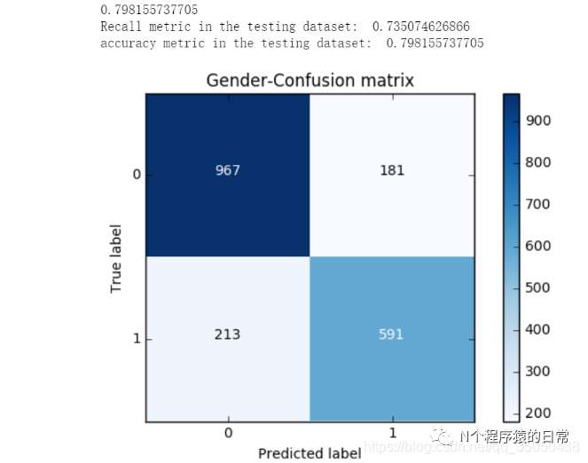

from sklearn.ensemble import RandomForestClassifierfrom sklearn.metrics import confusion_matrixfrom sklearn.cross_validation import train_test_splitX_train, X_test, y_train, y_test = train_test_split(gender_train,genderlabel,test_size = 0.2, random_state = 0)RF_model = RandomForestClassifier(n_estimators=100,min_samples_split=5,max_depth=10)RF_model.fit(X_train,y_train)
y_pred = RF_model.predict(X_test)print (RF_model.score(X_test,y_test))cnf_matrix = confusion_matrix(y_test,y_pred)print("Recall metric in the testing dataset: ", cnf_matrix[1,1]/(cnf_matrix[1,0]+cnf_matrix[1,1]))print("accuracy metric in the testing dataset: ", (cnf_matrix[1,1]+cnf_matrix[0,0])/(cnf_matrix[0,0]+cnf_matrix[1,1]+cnf_matrix[1,0]+cnf_matrix[0,1]))# Plot non-normalized confusion matrixclass_names = [0,1]
plt.figure()
plot_confusion_matrix(cnf_matrix, classes=class_names, title='Gender-Confusion matrix')
plt.show()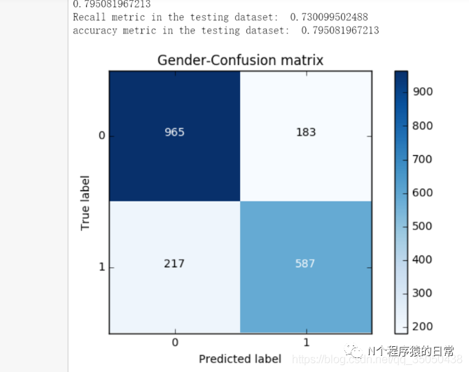

十：堆叠模型

from sklearn.svm import SVCfrom sklearn.naive_bayes import MultinomialNB
clf1 = RandomForestClassifier(n_estimators=100,min_samples_split=5,max_depth=10)
clf2 = SVC()
clf3 = LogisticRegression()
basemodes = [['rf', clf1],['svm', clf2],['lr', clf3]]

from sklearn.cross_validation import KFold, StratifiedKFold
models = basemodes#X_train, X_test, y_train, y_testfolds = list(KFold(len(y_train), n_folds=5, random_state=0))print (len(folds))
S_train = np.zeros((X_train.shape[0], len(models)))
S_test = np.zeros((X_test.shape[0], len(models)))for i, bm in enumerate(models):clf = bm[1]    #S_test_i = np.zeros((y_test.shape[0], len(folds)))for j, (train_idx, test_idx) in enumerate(folds):X_train_cv = X_train[train_idx]y_train_cv = y_train[train_idx]X_val = X_train[test_idx]clf.fit(X_train_cv, y_train_cv)y_val = clf.predict(X_val)[:]S_train[test_idx, i] = y_valS_test[:,i] = clf.predict(X_test)final_clf = RandomForestClassifier(n_estimators=100)
final_clf.fit(S_train,y_train)print (final_clf.score(S_test,y_test))